A common instinct in machine learning is: when prediction is hard, build a more powerful model. More features. A larger network. A richer representation. A more sophisticated objective.

That instinct works well when the target is close by. It works much worse on long-horizon problems, where the thing we can measure sits far downstream of the thing we control, and most of what moves it has nothing to do with us.

On those problems, the model is often struggling because we are asking it to predict far more than the decision actually requires. And a small amount of carefully designed intervention can give us information that changes the learning problem itself — often replacing a great deal of model capacity.

What long-horizon problems have in common

Consider three settings that look unrelated:

• An agentic LLM system. At some step the agent can call a tool, plan before acting, ask a clarifying question, retrieve more context, or spend more reasoning tokens. Whether the task ultimately succeeds is many steps away, and depends mostly on task difficulty, the environment, and the user.
• A recommender optimizing long-term value. A ranking change today affects retention months from now, alongside seasonality, content supply, and every other system in the product.
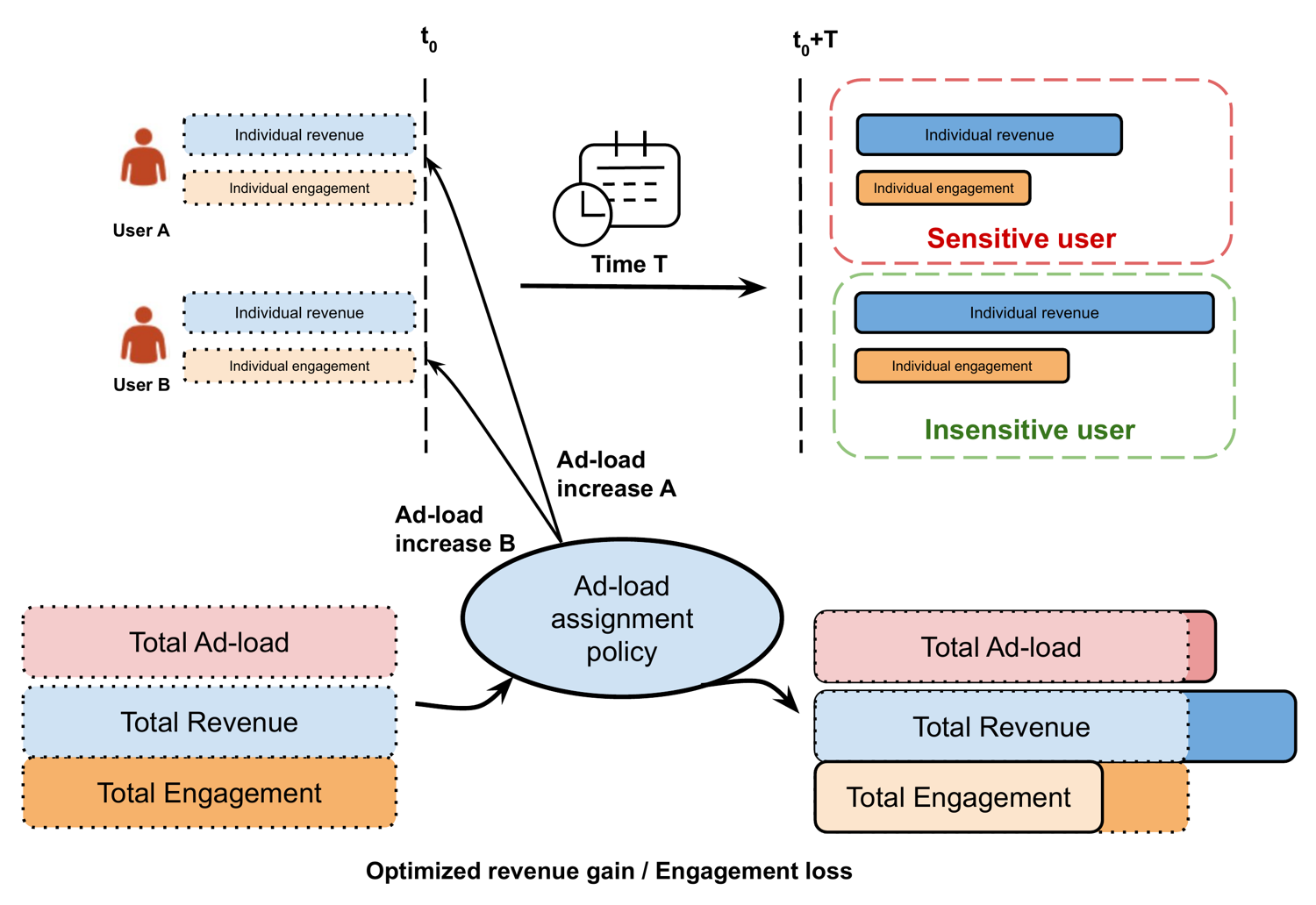
• An ads system adjusting how much advertising a user sees. More ads can raise revenue and lower long-term engagement, and the engagement effect only resolves over months.

The shared structure is this. We control a small intervention $W$. We care about an outcome $Y$ measured at a long horizon $T$. And $Y$ is dominated by variation we neither control nor observe.

Two consequences follow. First, predicting $Y$ well is extremely hard, and gets harder the longer we wait. Second — and this is the useful part — we usually do not need to predict $Y$ at all. We need to know how $Y$ changes when we intervene.

Throughout, I will use ads supply as the worked example, because it is the one where I can point at published numbers. The system and the figures come from Ads Supply Personalization via Doubly Robust Learning (CIKM ‘24). But nothing about the argument is specific to ads, and I will come back to the agentic case at the end.

The decision needs the consequence, not the outcome

Write the decision generically. For each unit $i$ (a user, a session, an agent trajectory) we choose $z_i \in {0,1}$: do we apply the intervention or not? We want the units where the benefit is large and the cost is small, subject to a budget on total cost.

In the ads instance, the benefit is incremental revenue and the cost is incremental engagement loss, which gives the knapsack problem from our paper:

Here $\tau^r(x_i)$ is the intervention’s incremental revenue effect, $\tau^e(x_i)$ is its incremental engagement effect, and $B$ is the allowable engagement-loss budget.

The important observation is what is not in this problem. Nowhere do we need to know how much revenue a user will generate over the next several months. We need to know how much that revenue will change because we intervened. Swap in an agentic system and the shape is identical: we do not need to predict whether a task will succeed, we need to know whether calling the tool makes success more likely, and what it costs.

Those are very different modeling problems.

Absolute outcomes are harder than intervention consequences

A long-horizon outcome might depend on seasonality, changes in user activity, new models shipped by other teams, product launches, content supply, macro events, and many latent factors we never observe.

The intervention we care about, meanwhile, is usually deliberately small. Conceptually:

The absolute outcome is complicated. The decision-relevant quantity is just:

Predicting both absolute outcomes accurately and subtracting them is a surprisingly expensive way to recover a small incremental effect. And the longer the horizon, the more unrelated variation accumulates, so the signal-to-noise ratio of the intervention effect keeps falling.

Potential outcomes versus the quantity we need

Under the potential-outcome framework, define the conditional average treatment effect (CATE):

A straightforward meta-learning strategy estimates the two potential outcomes separately:

This is natural, and it is also what a value model or reward model does implicitly when we use it to compare actions. But notice what it requires. If $\hat{Y}(X, 1)$ and $\hat{Y}(X, 0)$ both represent noisy, long-horizon outcomes, we need two good models of an extremely complicated target just to estimate their relatively small difference.

That leaves an awkward choice: accept weak treatment-effect estimates, or spend enormous model capacity predicting quantities we do not ultimately care about.

Model the intervention consequence, not the world

The treatment effect itself can be far more structured than either absolute outcome. Suppose the long-horizon outcome depends on hundreds of factors. Sensitivity to a small intervention may depend on many fewer — in the ads case, historical ad tolerance, activity level, engagement pattern, cohort, recent exposure.

Then the potential outcome

may be extremely complex, while

can still be relatively simple. Which suggests a different modeling philosophy: don’t model everything that determines the outcome if the decision only requires the consequence of your action.

A rough analogy is climate control. Predicting a building’s exact temperature tomorrow requires modeling weather, occupancy, sunlight, and ventilation. Estimating what happens to a room if you nudge the heater up is much easier. The state of the world is complicated; the local response to an intervention may not be.

The catch: the treatment effect has no label

We never observe $Y_i(1) - Y_i(0)$ for an individual unit. If it received treatment we see $Y_i = Y_i(1)$; otherwise $Y_i = Y_i(0)$. The other potential outcome is missing.

So although CATE may be the simpler function, it is not directly available as a supervised-learning target. This is where a small intervention budget becomes valuable.

An intervention gives us more than another dataset

Suppose we devote a small fraction of traffic to a randomized experiment. Most explanations stop at “an RCT removes confounding.” True, but there is a second benefit that gets less attention: we know the policy that generated the assignment.

For observational data, define the propensity score:

The assignment policy may itself be complicated, and we may need another large model just to estimate $e(x)$. But if we deliberately assign a fixed fraction $p$ to treatment, then $e(x) = p$. We do not estimate it. We know it.

The experiment has given us more than outcomes. It has given us information about how the data was generated, and that information is a form of supervision.

Conditional randomization becomes actual randomization

With observational data, identification usually relies on unconfoundedness:

After conditioning on $X$, treatment should behave as though randomized. An experiment gives the stronger condition:

Assignment no longer depends on potential outcomes, and because we designed it, the propensity is known. That combination gives us a way to compensate for an imperfect model of the absolute outcome.

Doubly robust estimation: let the experiment correct the model

Given an outcome predictor $\hat{Y}(X_i, W=t)$, a doubly robust estimate of the potential outcome is:

Then:

Two pieces. The first is what the model predicts. The second is a correction based on what actually happened under the known collection policy:

When the outcome model makes a mistake on an experimentally observed example, the residual tells us something about that mistake, and the propensity tells us how to weight it. The learner is no longer forced to trust the outcome model completely. The experiment can correct it.

From noisy outcome to treatment-effect pseudo-label

Doubly robust learning goes one step further. With known propensity $p$, construct the pseudo-outcome:

The second part,

is the model’s estimate of the intervention consequence. The first part,

uses the experimental assignment and the observed residual to correct that estimate.

This converts a difficult absolute-outcome prediction problem into a new supervised problem whose target is much closer to what the decision system needs. Finally, regress $\hat{\phi}(X)$ on $X$ to get the CATE model $M(X) \approx \tau(X)$ — explicitly separating nuisance prediction from intervention-consequence prediction.

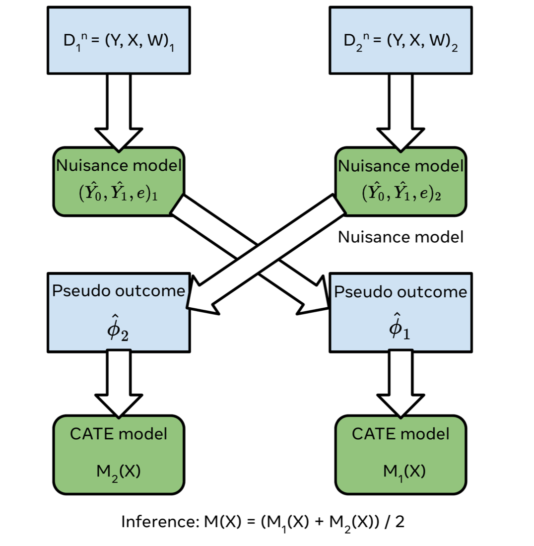
One detail worth noting: the training data is split in two, and the nuisance model fit on one subset builds the pseudo-outcome for the other. This cross-fitting keeps the nuisance model from having seen the examples whose residuals it is used to correct, and the two resulting CATE models are averaged at inference.

What happens when the outcome model is wrong

One experiment makes the payoff concrete. We deliberately inject increasing bias into the labels used to train the nuisance outcome model. If treatment-effect estimation depends strongly on predicting absolute outcomes correctly, performance should deteriorate. It does.

A T-learner estimates $\hat{\tau}(X) = \hat{Y}_1(X) - \hat{Y}_0(X)$; when both outcome models become biased, their difference does too. The doubly robust learner behaves very differently, because the known assignment policy keeps correcting residual errors.

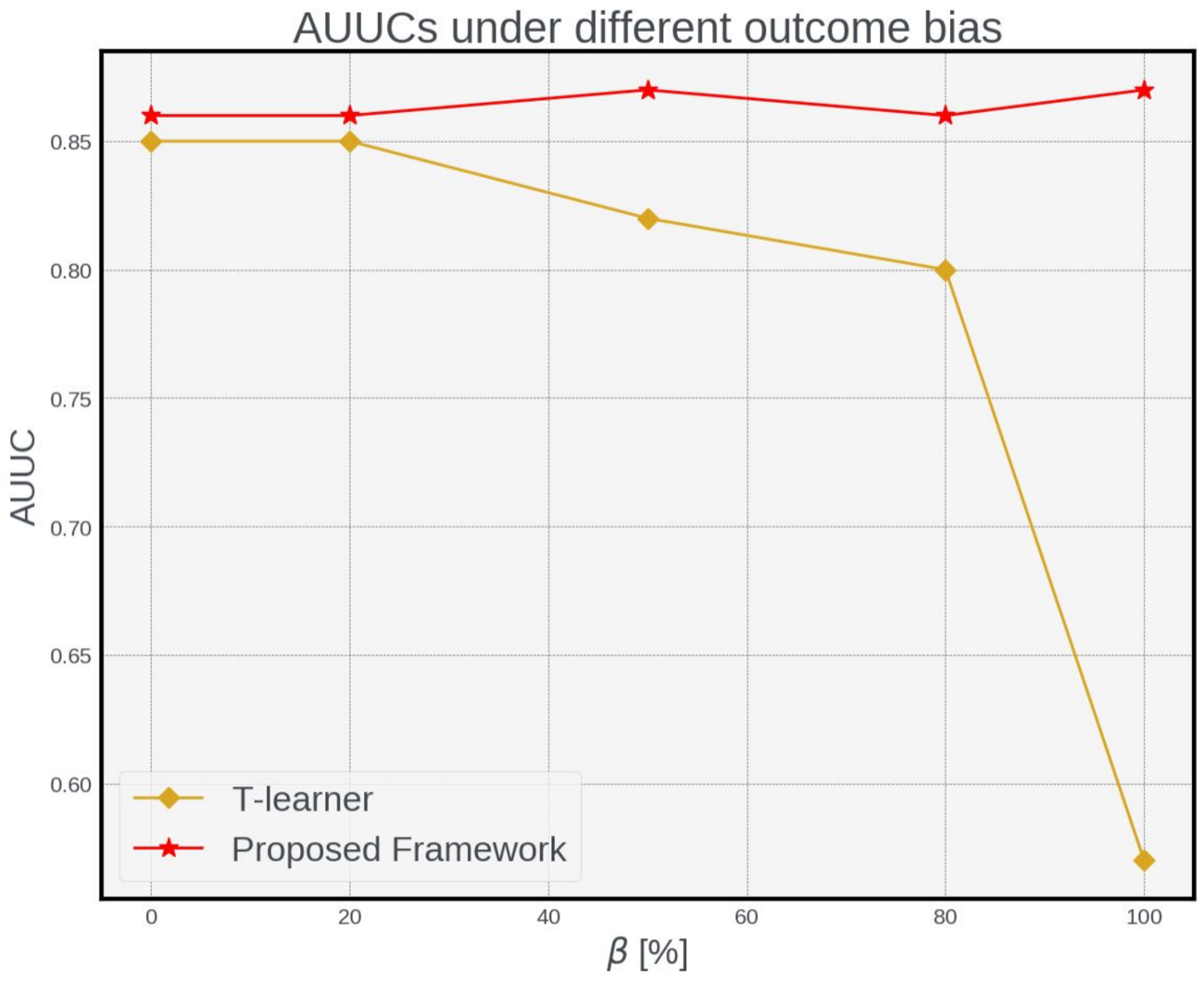
This is the property that matters for long horizons. The longer the horizon, the more likely the outcome model is misspecified — so the more valuable it is that our treatment-effect estimate does not depend on getting it right.

The honest caveat: bias is not the only thing that matters

It would be too convenient to stop there, because the long horizon cuts both ways.

The doubly robust estimator is unbiased, but it has higher variance than the direct estimator. And look at where that variance comes from: the correction term contains $Y - \hat{Y}(X, W)$, whose spread scales with the variance of the long-horizon outcome. The same property that makes the outcome model unreliable — enormous background variation in $Y$ — also inflates the variance of the correction meant to rescue us.

So the horizon helps the bias argument and hurts the variance argument simultaneously. What resolves the tension is scale. The variance penalty washes out as the dataset grows, which is why the framework’s advantage shows up most clearly in large-scale applications. Our data-size ablation makes the point directly: as the product dataset grows, the doubly robust framework’s AUCC improves while the T-learner’s stays flat. CATE estimates based solely on outcome predictions do not benefit from more data; the DR-derived model does.

The practical condition is therefore not “long horizon” alone but long horizon at scale. A long-horizon problem with a small sample is arguably the worst case: maximum outcome variance, not enough data to damp it.

A related caution: better outcome models still help. In our product data, swapping the nuisance model from a constant to a random forest to an MLP moved AUCC from 0.63 to 0.77 to 0.80. Improving it reduces DR variance even though it is not needed for consistency. The claim is “you don’t need the big model to be correct,” not “the outcome model stops mattering.”

Why a lightweight model becomes possible

Once outcome-model accuracy is no longer the dominant bottleneck, we do not need to deploy an enormous model simply because the raw outcome is complicated. In our implementation, both the nuisance models and the second-stage CATE regressor could use lightweight random forests.

The point was never that random forests beat deep networks. It was that if the statistical target and the data-generating process are designed correctly, we may no longer need the more complex model.

This matters at scale. A personalization model may need to score billions of units while sitting on top of already expensive ranking systems. Inference complexity is itself a product constraint, so reducing model complexity is not aesthetic — it decides whether a causal method can be deployed at all.

A small intervention budget changes the information structure

This suggests a different way to think about data budgets. Imagine dataset A with 100 million observational examples, and dataset B with 100,000 randomized ones. By sample count A dwarfs B, but their information is qualitatively different.

The observational dataset tells us a lot about the joint distribution $P(X, Y, W)$. The intervention dataset additionally tells us something unusually valuable about $P(W \mid X)$ — because we chose it — and randomization tells us assignment is independent of potential outcomes.

Those 100,000 samples are not merely another 100,000 labels. They encode knowledge about the mechanism that generated the labels, which can carry disproportionate statistical value.

Back to agentic tasks

Long-horizon credit assignment is exactly the problem agentic systems have, and the same structure applies.

Suppose we want to know whether calling a tool at a given step improves task success, whether planning first helps, whether asking a clarifying question is worth the turn, whether deeper retrieval pays for itself, or whether more reasoning tokens improve correctness.

The natural approach is to train a value or reward model to predict final task success, then compare its predictions across actions. That is the T-learner, and it inherits the T-learner’s failure mode: final success over a long trajectory is dominated by task difficulty, environment variation, and user behavior, so a model good enough to predict it is enormously expensive — and small errors in two large predictions swamp the difference we actually wanted.

The alternative is to spend a small intervention budget. Hold the trajectory fixed up to a decision point and deliberately randomize the action: call the tool or don’t, plan or don’t, retrieve three documents or ten. Then measure the incremental consequence. Instead of asking a huge model to infer the effect from whatever correlations appear in naturally generated data, the intervention exposes the contrast directly.

And the propensity analogue is already sitting in the logs. Sampling temperature, exploration probability, which policy variant served a trajectory, how an A/B assignment was made — these are known, not estimated. Discarding them and treating every trajectory as an ordinary supervised example throws away information the system already has.

This is the same trap I wrote about in a previous post from the other direction: a reward model trained to predict what accompanies good outcomes gets used to decide what the policy should produce more of. Prediction and intervention are different questions, and a long horizon widens the gap between them.

The caveat carries over too. Long agentic trajectories have enormous outcome variance, so the correction term is noisy, and this approach wants scale to pay off.

Spend intervention budget where information is missing

Once intervention is expensive, the next question is where to intervene. Not every region of the distribution is equally uncertain. Intervention is most valuable where treatment overlap is poor, where causal models disagree, where estimated effects have high uncertainty, where the decision has high downstream value, or where observational data cannot distinguish competing explanations.

That suggests an adaptive loop: start from observational data, estimate effects and their uncertainty, identify high-value uncertainty, target the intervention budget there, update the effect model, repeat.

Experimentation then becomes active information acquisition. The system is not simply consuming whatever data production happens to generate — it is deciding which additional evidence would most improve the decision.

The data-collection policy is part of the model

We usually think of an ML system as a pipeline from dataset to model to decision. A more complete picture closes the loop:

The policy that generated the data is not incidental metadata. It is part of the statistical information available to the learner. In the ads case, randomized assignment gave us a known propensity score. In a general system, the learner may know the exploration probability, the logging policy, the sampling strategy, or the intervention intensity.

But the future is not experiments versus observational data

Interventions are expensive. They consume revenue, user experience, experimentation capacity, and engineering time — and on long-horizon problems they also consume time, since you cannot shortcut the measurement window. So the conclusion cannot be “randomize everything.”

Observational data, meanwhile, is nearly free and enormously abundant, giving population coverage, rich representations, rare contexts, and natural behavior.

The two are complementary. Observational data is good for learning what the world looks like; intervention data is good for learning what changes when I act. The optimal system should not ask one source to do the other’s job. Abundant observational data plus a small, high-information intervention set can beat either alone.

Final takeaway

The lesson was not that experimental data is better than observational data. It was more specific: a small intervention budget changes the learning problem in three ways.

1. It lets us model the quantity the decision actually needs. Instead of predicting noisy absolute outcomes $Y(0)$ and $Y(1)$, the final learner targets

2. It gives us information about the data-generation mechanism. Because we control assignment, $e(X) = p$ is known rather than estimated.

3. Doubly robust learning combines the two. The known collection policy and the observed residuals build a pseudo-outcome

from which a lightweight model learns the intervention consequence directly.

With the caveat that this trades bias for variance, so it wants scale — and that on long-horizon problems, where the trade is most attractive, the variance is also largest.

Modern ML is extraordinarily good at two kinds of scaling: more model, and more data. There is a third axis — more informative data. A thousand well-chosen interventions can sometimes answer a question that millions of passive observations cannot. Samples have different information value depending on how they were generated.

So the goal is not to maximize the number of observations. It is to maximize decision-relevant information per unit of data-collection cost. Or more simply: don’t ask a model to reconstruct information you can obtain more cheaply by changing the data-generating process. Don’t only scale the learner — scale the information in the learning problem.